Eigenvalues and eigenvectors

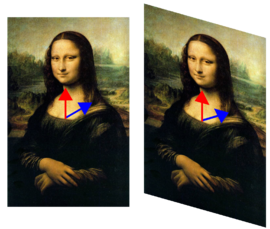
In this shear mapping of the Mona Lisa, the picture was deformed in such a way that its central vertical axis (red vector) has not changed direction, but the diagonal vector (blue) has changed direction. Hence the red vector is an eigenvector of the transformation and the blue vector is not. Since the red vector was neither stretched nor compressed, its eigenvalue is 1. All vectors with the same or opposite direction (vertical upward or downward) are also eigenvectors, and have the same eigenvalue. Together with the zero vector, they form the eigenspace for this eigenvalue.

The eigenvectors of a square matrix are the non-zero vectors which, after being multiplied by the matrix, continue to point in either the same direction or in the opposite direction. For each eigenvector, the corresponding eigenvalue is the factor by which the eigenvector changes its length when multiplied by the matrix. A vector that points in the opposite direction after being multiplied by the matrix has a negative eigenvalue. The prefix eigen- is adopted from the German word "eigen" for "innate", "own".^[1] The eigenvectors are sometimes also called proper vectors, or characteristic vectors. Similarly, the eigenvalues are also known as proper values, or characteristic values.

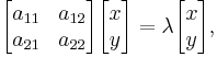
Formally and more generally, if A is a linear transformation, which may or may not be represented by a square matrix, a non-zero vector x is an eigenvector of A if there is a scalar λ such that

$A\mathbf{x} = \lambda \mathbf{x} \, .$

The scalar λ is said to be the eigenvalue of A corresponding to x.

An eigenspace of A is the set of all eigenvectors with the same eigenvalue. By convention, the zero vector, while not an eigenvector, is also a member of every eigenspace. For a fixed λ

$\{ \mathbf{x} | A\mathbf{x} = \lambda \mathbf{x} \}$

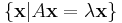
is an eigenspace of A.

Eigenvalues and eigenvectors have many applications in both pure and applied mathematics. They are used in matrix factorization, in quantum mechanics, and in many other areas.

1 Overview
2 Mathematical definition
- 2.1 Alternative definition
3 Computation of eigenvalues and eigenvectors
4 Properties of eigenvectors
5 Properties of eigenvalues
6 Left and right eigenvectors
7 History
8 Existence and multiplicity
9 Infinite-dimensional spaces and spectral theory
- 9.1 Eigenfunctions
  - 9.1.1 Waves on a string
10 Eigendecomposition
11 Applications
12 See also
13 Notes
14 References
15 External links

Overview

In linear algebra, there are three kinds of objects:

scalars, which are just numbers;
vectors, which can be thought of as arrows, and which have both length (or magnitude) and direction (though more precisely a vector is a member of a vector space);
matrices, which are arrays of numbers arranged in rows and columns.

In place of the ordinary functions of algebra, the most important functions in linear algebra are called linear transformations, and a linear transformation of a vector is a change in the vector, usually performed by means of a matrix. Thus instead of writing f(x) we write M(v) or simply Mv, where M is a matrix and v is a vector. The rules for using a matrix to transform a vector are given in the article linear algebra.

In general, a square matrix can only change the magnitude and/or direction of the vector upon which it acts. If the action of a matrix on a (nonzero) vector changes its magnitude but not its direction, then the vector is called an eigenvector of that matrix. There are infinitely many eigenvectors having the same or an opposite direction, and there may exist eigenvectors in other directions. When transformed by the matrix, each of these eigenvector changes its magnitude by a factor, called the eigenvalue corresponding to that eigenvector. The eigenspace corresponding to one eigenvalue of a given matrix is the set of all eigenvectors of the matrix with that eigenvalue. A matrix may have more than one eigenvalue (and hence more than one eigenspace). The set of eigenvalues for a given matrix M is sometimes called the spectrum of M (the maximum number of eigenvalues is the same as the number of dimensions of the vector space in which v belongs, and on which M operates).

An important benefit of knowing the eigenvectors and eigenvalues of a system is that the effects of the action of the matrix on the system can be predicted. Each application of the matrix to an arbitrary vector yields a result which will have rotated towards the eigenvector with the largest eigenvalue. ^[2]

Many kinds of mathematical objects can be treated as vectors: ordered pairs, functions, harmonic modes, quantum states, and frequencies are examples. In these cases, the concept of direction loses its ordinary meaning, and is given an abstract definition. Even so, if this abstract direction is unchanged by a given linear transformation, the prefix "eigen" is used, as in eigenfunction, eigenmode, eigenface, eigenstate, and eigenfrequency.

Mathematical definition

Definition	Given a linear transformation A, a non-zero vector x is defined to be an eigenvector of the transformation if it satisfies the eigenvalue equation $A\, \mathbf{x} = \lambda\, \mathbf{x}$ for some scalar λ. In this situation, the scalar λ is called an eigenvalue of A corresponding to the eigenvector x.^[3]

Transformation A acts to stretch the vector x, not change its direction, so x is an eigenvector of A.

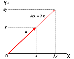
Key to this definition is the eigenvalue equation, Ax = λx. The vector x has the property that its direction is not changed by the transformation A, but that it is only scaled by a factor of λ. Most vectors x will not satisfy such an equation: a typical vector x changes direction when acted on by A, so that Ax is not a scalar multiple of x. This means that only certain special vectors x are eigenvectors, and only certain special scalars λ are eigenvalues. Of course, if A is a multiple of the identity matrix, then no vector changes direction, and all non-zero vectors are eigenvectors.

Geometrically, the eigenvalue equation means that under the transformation A eigenvectors experience only changes in magnitude and sign—the direction of Ax is either the same as that of x, or its opposite. The eigenvalue λ is simply the amount of "stretch" or "shrink" to which a vector is subjected when transformed by A. If λ = 1, the vector remains unchanged (unaffected by the transformation). A transformation I under which a vector x remains unchanged, Ix = x, is defined as identity transformation. If λ = −1, the vector flips to the opposite direction; this is defined as reflection.

Notice that the eigenvalue equation Ax = λx implies that A must be a square matrix, and its size must be n-by-n (n rows and n columns), where n is the number of dimensions of the vector space in which x is contained. Otherwise, the transformation would always produce a vector in a different vector space (different from λx).

Alternative definition

Mathematicians sometimes alternatively define eigenvalue in the following way, leading to differences of opinion over what constitutes an "eigenvector."

Alternative Definition	Given a linear transformation A on a linear space V over a field F, a scalar λ in F is called an eigenvalue of A if there exists a nonzero vector x in V such that $A\, \mathbf{x} = \lambda\, \mathbf{x}$ Any vector u in V which satisfies $A\, \mathbf{u} = \lambda\, \mathbf{u}$ for some eigenvalue λ is called an eigenvector of A corresponding to λ. The set of all eigenvectors corresponding to λ is called the eigenspace of λ.^[4]

Notice that the above definitions are entirely equivalent, except for in regards to eigenvectors, where they disagree on whether the zero vector is considered an eigenvector. The convention of allowing the zero vector to be an eigenvector (although still not allowing it to determine eigenvalues) allows one to avoid repeating the non-zero criterion every time one proves a theorem, and simplifies the definitions of concepts such as eigenspace, which would otherwise be non-intuitively made up of vectors that are not all eigenvectors.

Computation of eigenvalues and eigenvectors

To compute the eigenvectors of a matrix, we first compute its eigenvalues. It is not always easy to compute eigenvalues, but when they are known, it is relatively easy to compute the corresponding eigenvectors.

Eigenvalues

When a transformation is represented by a square matrix A, the eigenvalue equation can be expressed as

$A \mathbf{x} - \lambda I \mathbf{x} = \mathbf{0} \, ,$

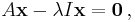
where I is the identity matrix. This can be rearranged to

$(A - \lambda I) \mathbf{x} = \mathbf{0} \, .$

If there exists an inverse

$\displaystyle(A - \lambda I)^{-1},$

then both sides can be left multiplied by the inverse to obtain the trivial solution: x = 0. Thus we require there to be no inverse by assuming from linear algebra that the determinant equals zero:

$\det(A - \lambda I) = 0\, .$

The determinant requirement is called the characteristic equation (less often, secular equation) of A, and the left-hand side is called the characteristic polynomial. When expanded, this gives a polynomial equation for $\lambda$ . Neither the eigenvector x nor its components are present in the characteristic equation.

This characteristic equation will have N_λ distinct solutions, where 1 ≤ N_λ ≤ N, where N is the number of dimensions of the vector space in which x is contained. The set of solutions, i.e. the eigenvalues, is sometimes called the spectrum of A.

Eigenvectors

Based on the eigenvalues, the corresponding eigenvectors can be computed by solving for each eigenvalue λ_i, the equation

$A\, \mathbf{x} = \lambda_i\, \mathbf{x}$

For each eigenvalue, λ_i, we have a specific eigenvalue equation. There will be 1 ≤ m_i ≤ n_i linearly independent solutions to each eigenvalue equation. The m_i solutions are the eigenvectors associated with the eigenvalue λ_i. The integer m_i is termed the geometric multiplicity of λ_i. It is important to keep in mind that the algebraic multiplicity n_i and geometric multiplicity m_i may or may not be equal, but we always have m_i ≤ n_i. The simplest case is of course when m_i = n_i = 1. The total number of linearly independent eigenvectors, N_x, can be calculated by summing the geometric multiplicities

$\sum\limits_{i=1}^{N_{\lambda}}{m_i} =N_{\mathbf{x}}.$

The eigenvectors can be indexed by eigenvalues, i.e. using a double index, with x_i,j being the j^th eigenvector for the i^th eigenvalue. The eigenvectors can also be indexed using the simpler notation of a single index x_k, with k = 1, 2, ... , N_x.

Example 1

The matrix

$\begin{bmatrix} 2 & 1\\1 & 2 \end{bmatrix}$

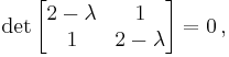
defines a linear transformation of the real plane. The eigenvalues of this transformation are given by the characteristic polynomial

$\det\begin{bmatrix} 2-\lambda & 1\\1 & 2-\lambda \end{bmatrix} = 0 \, ,$

$\Rightarrow (2-\lambda)^2 - 1 = 0 \, ,$

$\Rightarrow \lambda^2 - 4 \lambda + 3 = 0 \, .$

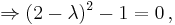
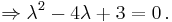
The roots of this polynomial (i.e. the values of $\lambda$ for which the equation holds) are $\lambda=1$ and $\lambda=3$ . Having found the eigenvalues, it is possible to find the eigenvectors. Considering first the eigenvalue $\lambda=3$ , we have

$\begin{bmatrix} 2 & 1\\1 & 2 \end{bmatrix}\begin{bmatrix}x\\y\end{bmatrix} = 3 \begin{bmatrix}x\\y\end{bmatrix}.$

After matrix-multiplication

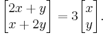
$\begin{bmatrix} 2x+y \\x+2y \end{bmatrix} = 3 \begin{bmatrix}x\\y\end{bmatrix}.$

This matrix equation represents a system of two linear equations $2x+y=3x$ and $x+2y=3y$ . Both the equations reduce to the single linear equation $x=y$ . To find an eigenvector, we are free to choose any value for x (except 0), so by picking x=1 and setting y=x, we find an eigenvector with eigenvalue 3 to be

$\begin{bmatrix}1\\1\end{bmatrix}.$

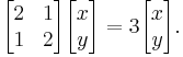
We can confirm this is an eigenvector with eigenvalue 3 by checking the action of the matrix on this vector:

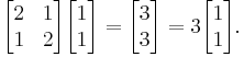
$\begin{bmatrix}2&1\\1&2\end{bmatrix}\begin{bmatrix}1\\1\end{bmatrix} = \begin{bmatrix}3\\3\end{bmatrix} = 3\begin{bmatrix}1\\1\end{bmatrix}.$

Any scalar multiple of this eigenvector will also be an eigenvector with eigenvalue 3.

For the eigenvalue $\lambda=1,$ a similar process leads to the equation $x=-y$ , and hence an eigenvector with eigenvalue 1 is given by

$\begin{bmatrix}1\\-1\end{bmatrix}.$

The complexity of the problem for finding roots/eigenvalues of the characteristic polynomial increases rapidly with increasing the degree of the polynomial (the dimension of the vector space). There are exact solutions for dimensions below 5, but for dimensions greater than or equal to 5 there are generally no exact solutions and one has to resort to numerical methods to find them approximately. Worse, this computational procedure can be very inaccurate in the presence of round-off error, because the roots of a polynomial are an extremely sensitive function of the coefficients (see Wilkinson's polynomial).^[5] Efficient, accurate methods to compute eigenvalues and eigenvectors of arbitrary matrices were not known until the advent of the QR algorithm in 1961.^[5] For large Hermitian sparse matrices, the Lanczos algorithm is one example of an efficient iterative method to compute eigenvalues and eigenvectors, among several other possibilities.^[5]

Example 2

If a matrix is a n-by-n diagonal matrix, then its eigenvalues are the numbers on the diagonal and its eigenvectors are the n unit vectors forming the standard basis for the n-dimensional vector space on which the matrix operates. For example, the matrix

$\begin{bmatrix} 3 & 0\\ 0 & 0.5\end{bmatrix}$

which operates on a two-dimensional space, stretches every vector in the x-direction to three times its original length, and shrinks every vector in the y-direction to half its original length. Eigenvectors corresponding to the eigenvalue 3 are any multiple of the basis vector [1, 0]; together they constitute the eigenspace corresponding to the eigenvalue 3. Eigenvectors corresponding to the eigenvalue 0.5 are any multiple of the basis vector [0, 1]; together they constitute the eigenspace corresponding to the eigenvalue 0.5.

In contrast, any other vector, [2, 8] for example, will change direction. The angle [2, 8] makes with the x-axis has tangent 4, but after being transformed, [2, 8] is changed to [6, 4], and the angle that vector makes with the x-axis has tangent 2/3.

Properties of eigenvectors

Non-zero values

The requirement that the eigenvector be non-zero is imposed because the equation A0 = λ0 holds for every A and every λ. Since the equation is always trivially true, it is not an interesting case. In contrast, an eigenvalue can be zero in a nontrivial way. Each eigenvector is associated with a specific eigenvalue. One eigenvalue is associated with an infinite number of eigenvectors that span, at least, a one-dimensional eigenspace, as follows.

Scalar multiples

If x is an eigenvector of the linear transformation A with eigenvalue λ, then any scalar multiple αx is also an eigenvector of A with the same eigenvalue, since A(αx) = αAx = αλx = λ(αx). The set of all such eigenvectors belonging to the same scaling factor, λ, is called an eigenline.

More generally, any linear combination of eigenvectors that share the same eigenvalue λ, will itself be an eigenvector with eigenvalue λ.^[6] Together with the zero vector, the eigenvectors of A with the same eigenvalue form a linear subspace of the vector space called an eigenspace, E_λ. In case of dim(E_λ) = 1, it is called an eigenline and λ is called a scaling factor.

Components of eigenvectors

If a basis is defined in vector space, all vectors can be expressed in terms of components. For finite dimensional vector spaces with dimension n, linear transformations can be represented with n × n square matrices. Conversely, every such square matrix corresponds to a linear transformation for a given basis. Thus, in a two-dimensional vector space R² fitted with standard basis, the eigenvector equation for a linear transformation A can be written in the following matrix representation:

$\begin{bmatrix} a_{11} & a_{12} \\ a_{21} & a_{22} \end{bmatrix} \begin{bmatrix} x \\ y \end{bmatrix} = \lambda \begin{bmatrix} x \\ y \end{bmatrix},$

where the juxtaposition of matrices denotes matrix multiplication.

Since, by definition of λ, det(λI-A)=0, the solution is not unique — at least one coordinate is a free variable. This results in a whole dimension of λ-associated eigenvectors, as explained in the property above.

Linear independence

The eigenvectors corresponding to different eigenvalues are linearly independent^[7] meaning, in particular, that in an n-dimensional space the linear transformation A cannot have more than n eigenvalues (or eigenspaces).^[8]

A matrix is said to be defective if it fails to have n linearly independent eigenvectors. All defective matrices have fewer than n distinct eigenvalues, but not all matrices with fewer than n distinct eigenvalues are defective.^[9]

Eigenvectors of a diagonal matrix

If a matrix is a diagonal matrix, then its eigenvalues are the numbers on the diagonal and its eigenvectors are basis vectors (of the standard basis) to which those numbers refer.

Properties of eigenvalues

Let $A$ be an n×n matrix with eigenvalues $\lambda_i$ , $i=1,2,\dots,n$ . Then

Trace of $A= \lambda_1+ \lambda_2 +\cdots+ \lambda_n$ .
Determinant of $A=\lambda_1\lambda_2\cdots\lambda_n$ .
Eigenvalues of $A^k$ are $\lambda_1^k,\dots,\lambda_n^k$
If $A=A^H$ , i.e., $A$ is Hermitian, every eigenvalue is real.
Every eigenvalue of a Unitary matrix has absolute value $|\lambda|=1$ .

Left and right eigenvectors

The word eigenvector formally refers to the right eigenvector $x_R$ . It is defined by the above eigenvalue equation

$A x_R = \lambda_R x_R,\$

and is the most commonly used eigenvector. However, the left eigenvector $x_L$ exists as well, and is defined by

$x_L A = \lambda_L x_L. \$

History

Eigenvalues are often introduced in the context of linear algebra or matrix theory. Historically, however, they arose in the study of quadratic forms and differential equations.

Euler studied the rotational motion of a rigid body and discovered the importance of the principal axes. Lagrange realized that the principal axes are the eigenvectors of the inertia matrix.^[10] In the early 19th century, Cauchy saw how their work could be used to classify the quadric surfaces, and generalized it to arbitrary dimensions.^[11] Cauchy also coined the term racine caractéristique (characteristic root) for what is now called eigenvalue; his term survives in characteristic equation.^[12]

Fourier used the work of Laplace and Lagrange to solve the heat equation by separation of variables in his famous 1822 book Théorie analytique de la chaleur.^[13] Sturm developed Fourier's ideas further and brought them to the attention of Cauchy, who combined them with his own ideas and arrived at the fact that real symmetric matrices have real eigenvalues.^[11] This was extended by Hermite in 1855 to what are now called Hermitian matrices.^[12] Around the same time, Brioschi proved that the eigenvalues of orthogonal matrices lie on the unit circle,^[11] and Clebsch found the corresponding result for skew-symmetric matrices.^[12] Finally, Weierstrass clarified an important aspect in the stability theory started by Laplace by realizing that defective matrices can cause instability.^[11]

In the meantime, Liouville studied eigenvalue problems similar to those of Sturm; the discipline that grew out of their work is now called Sturm–Liouville theory.^[14] Schwarz studied the first eigenvalue of Laplace's equation on general domains towards the end of the 19th century, while Poincaré studied Poisson's equation a few years later.^[15]

At the start of the 20th century, Hilbert studied the eigenvalues of integral operators by viewing the operators as infinite matrices.^[16] He was the first to use the German word eigen to denote eigenvalues and eigenvectors in 1904, though he may have been following a related usage by Helmholtz. For some time, the standard term in English was "proper value", but the more distinctive term "eigenvalue" is standard today.^[17]

The first numerical algorithm for computing eigenvalues and eigenvectors appeared in 1929, when Von Mises published the power method. One of the most popular methods today, the QR algorithm, was proposed independently by John G.F. Francis^[18] and Vera Kublanovskaya^[19] in 1961.^[20]

Existence and multiplicity

For a given matrix, the number of eigenvalues and eigenvectors and whether they are distinct depends on properties of that matrix.

The algebraic multiplicity of an eigenvalue is defined as the multiplicity of the corresponding root of the characteristic polynomial. The geometric multiplicity of an eigenvalue is defined as the dimension of the associated eigenspace, i.e. number of linearly independent eigenvectors with that eigenvalue.

For transformations on real vector spaces, the coefficients of the characteristic polynomial are all real. However, the roots are not necessarily real; they may include complex numbers with a non-zero imaginary component. For example, a matrix representing a planar rotation of 45 degrees will not leave any non-zero vector pointing in the same direction.

However, over a complex vector space, the fundamental theorem of algebra guarantees that the characteristic polynomial has at least one root, and thus the linear transformation has at least one eigenvalue. Over a complex space, the sum of the algebraic multiplicities will equal the dimension of the vector space, but the sum of the geometric multiplicities may be smaller. In a sense, it is possible that there may not be sufficient eigenvectors to span the entire space. This is intimately related to the question of whether a given matrix may be diagonalized by a suitable choice of coordinates.

As well as distinct roots, the characteristic equation may also have repeated roots. However, having repeated roots does not imply there are multiple distinct (i.e., linearly independent) eigenvectors with that eigenvalue.

These concepts are illustrated by considering several common geometric transformations.

Shear

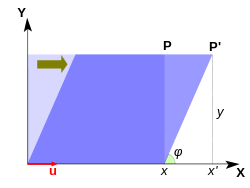
Horizontal shear. The shear angle φ is given by k = cot φ, where k is the shear factor

Shear in the plane is a transformation in which all points along a given line remain fixed while other points are shifted parallel to that line by a distance proportional to their perpendicular distance from the line.^[21] Shearing a plane figure does not change its area. Shear can be horizontal − along the X axis, or vertical − along the Y axis. In horizontal shear (see figure), a point P of the plane moves parallel to the X axis to the place P' so that its coordinate y does not change while the x coordinate increments to become x' = x + k y, where k is called the shear factor.

The matrix of a horizontal shear transformation is

$\begin{bmatrix}1 & k\\ 0 & 1\end{bmatrix}$ .

The characteristic equation is

$\lambda^2 - 2\lambda+1 = (1-\lambda)^2 = 0$

which has a single, repeated root λ = 1. Therefore, the eigenvalue λ = 1 has algebraic multiplicity 2. The eigenvector(s) are found as solutions of

$\begin{bmatrix}1 & k\\ 0 & 1\end{bmatrix} \begin{bmatrix}x\\ y\end{bmatrix} = \lambda \begin{bmatrix}x\\ y\end{bmatrix} \Rightarrow \begin{bmatrix}x + ky\\ y\end{bmatrix} = \begin{bmatrix}x\\ y\end{bmatrix} \Rightarrow \begin{bmatrix}x + ky\\ y\end{bmatrix} - \begin{bmatrix}x\\ y\end{bmatrix} = \begin{bmatrix}0\\ 0\end{bmatrix} \Rightarrow \begin{bmatrix}ky\\ 0\end{bmatrix} = \begin{bmatrix}0\\ 0\end{bmatrix} \, .$

The last equation is equivalent to y = 0, which is a straight line along the x axis. This line represents the one-dimensional eigenspace. In the case of shear the algebraic multiplicity of the eigenvalue (2) is greater than its geometric multiplicity (1, the dimension of the eigenspace). The eigenvector is a vector along the x axis. The case of vertical shear with transformation matrix $\begin{bmatrix}1 & 0\\ k & 1\end{bmatrix}$ is dealt with in a similar way; the eigenvector in vertical shear is along the y axis. Applying repeatedly the shear transformation changes the direction of any vector in the plane closer and closer to the direction of the eigenvector.

Uniform scaling and reflection

When a surface is stretching equally in all directions (a homothety) each of the radial vectors is an eigenvector.

As a one-dimensional vector space, consider an elastic string or rubber band tied to an unmoving support at one end. Pulling the string away from the point of attachment stretches it and elongates it by some scaling factor λ which is a real number. Each vector on the string is stretched equally, with the same scaling factor λ, and although elongated, it preserves its original direction.

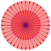
For a two-dimensional vector space, consider a rubber sheet stretched equally in all directions such as a small area of the surface of an inflating balloon. All vectors originating at the fixed point on the balloon surface (the origin) are stretched equally with the same scaling factor λ. This transformation in two dimensions is described by the 2×2 square matrix:

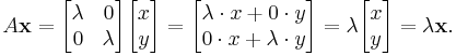
$A \mathbf{x} = \begin{bmatrix}\lambda & 0\\0 & \lambda\end{bmatrix} \begin{bmatrix} x \\ y \end{bmatrix} = \begin{bmatrix}\lambda \cdot x + 0 \cdot y \\0 \cdot x + \lambda \cdot y\end{bmatrix} = \lambda \begin{bmatrix} x \\ y \end{bmatrix} = \lambda \mathbf{x}.$

Expressed in words, the transformation is equivalent to multiplying the length of any vector by λ while preserving its original direction. Since the vector taken was arbitrary, every non-zero vector in the vector space is an eigenvector. Whether the transformation is stretching (elongation, extension, inflation), or shrinking (compression, deflation) depends on the scaling factor: if λ > 1, it is stretching; if λ < 1, it is shrinking. Negative values of λ correspond to a reversal of direction, followed by a stretch or a shrink, depending on the absolute value of λ.

Unequal scaling

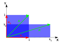
Vertical shrink (k₂ < 1) and horizontal stretch (k₁ > 1) of a unit square. Eigenvectors are u₁ and u₂ and eigenvalues are λ₁ = k₁ and λ₂ = k₂. This transformation orients all vectors towards the principal eigenvector u₁.

For a slightly more complicated example, consider a sheet that is stretched unequally in two perpendicular directions along the coordinate axes, or, similarly, stretched in one direction, and shrunk in the other direction. In this case, there are two different scaling factors: k₁ for the scaling in direction x, and k₂ for the scaling in direction y. The transformation matrix is

$\begin{bmatrix}k_1 & 0\\0 & k_2\end{bmatrix}$ ,

and the characteristic equation is

$(k_1-\lambda)(k_2-\lambda) = 0$ .

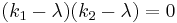The eigenvalues, obtained as roots of this equation are λ₁ = k₁, and λ₂ = k₂ which means, as expected, that the two eigenvalues are the scaling factors in the two directions. Plugging k₁ back in the eigenvalue equation gives one of the eigenvectors:

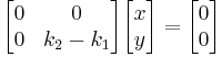$\begin{bmatrix}0 & 0\\0 & k_2 - k_1\end{bmatrix} \begin{bmatrix} x \\ y\end{bmatrix} = \begin{bmatrix}0\\0\end{bmatrix}$ or, more simply, $y=0$ .

Thus, the eigenspace is the x-axis. Similarly, substituting $\lambda=k_2$ shows that the corresponding eigenspace is the y-axis. In this case, both eigenvalues have algebraic and geometric multiplicities equal to 1. If a given eigenvalue is greater than 1, the vectors are stretched in the direction of the corresponding eigenvector; if less than 1, they are shrunken in that direction. Negative eigenvalues correspond to reflections followed by a stretch or shrink. In general, matrices that are diagonalizable over the real numbers represent scalings and reflections: the eigenvalues represent the scaling factors (and appear as the diagonal terms), and the eigenvectors are the directions of the scalings.

The figure shows the case where $k_1>1$ and $1>k_2>0$ . The rubber sheet is stretched along the x axis and simultaneously shrunk along the y axis. After repeatedly applying this transformation of stretching/shrinking many times, almost any vector on the surface of the rubber sheet will be oriented closer and closer to the direction of the x axis (the direction of stretching). The exceptions are vectors along the y-axis, which will gradually shrink away to nothing.

Rotation

For more details on this topic, see Rotation matrix.

A rotation in a plane is a transformation that describes motion of a vector, plane, coordinates, etc., around a fixed point. Clearly, for rotations other than through 0° and 180°, every vector in the real plane will have its direction changed, and thus there cannot be any eigenvectors. But this is not necessarily true if we consider the same matrix over a complex vector space.

A counterclockwise rotation in the horizontal plane about the origin at an angle φ is represented by the matrix

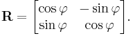
$\mathbf{R} = \begin{bmatrix} \cos \varphi & -\sin \varphi \\ \sin \varphi & \cos \varphi \end{bmatrix}.$

The characteristic equation of R is λ² − 2λ cos φ + 1 = 0. This quadratic equation has a discriminant D = 4 (cos² φ − 1) = − 4 sin² φ, which is a negative number whenever φ is not equal to a multiple of 180°. A rotation of 0°, 360°, … is just the identity transformation (a uniform scaling by +1), while a rotation of 180°, 540°, …, is a reflection (uniform scaling by -1). Otherwise, as expected, there are no real eigenvalues or eigenvectors for rotation in the plane.

Rotation matrices on complex vector spaces

The characteristic equation has two complex roots λ₁ and λ₂. If we choose to think of the rotation matrix as a linear operator on the complex two dimensional vector, we can consider these complex eigenvalues. The roots are complex conjugates of each other: λ_1,2 = cos φ ± i sin φ = e ^{± iφ}, each with an algebraic multiplicity equal to 1, where i is the imaginary unit.

The first eigenvector is found by substituting the first eigenvalue, λ₁, back into the eigenvalue equation:

$\begin{bmatrix} \cos \varphi - \lambda_1 & -\sin \varphi \\ \sin \varphi & \cos \varphi - \lambda_1 \end{bmatrix} \begin{bmatrix} x \\ y \end{bmatrix} = \begin{bmatrix} - i \sin \varphi & -\sin \varphi \\ \sin \varphi & - i \sin \varphi \end{bmatrix} \begin{bmatrix} x \\ y \end{bmatrix} = \begin{bmatrix} 0 \\ 0 \end{bmatrix}.$

The last equation is equivalent to the single equation $x=iy$ , and again we are free to set $x=1$ to give the eigenvector

$\begin{bmatrix}1\\-i\end{bmatrix}.$

Similarly, substituting in the second eigenvalue gives the single equation $x=-iy$ and so the eigenvector is given by

$\begin{bmatrix}1\\i\end{bmatrix}.$

Although not diagonalizable over the reals, the rotation matrix is diagonalizable over the complex numbers, and again the eigenvalues appear on the diagonal. Thus rotation matrices acting on complex spaces can be thought of as scaling matrices, with complex scaling factors.

Infinite-dimensional spaces and spectral theory

For more details on this topic, see Spectral theorem.

If the vector space is an infinite dimensional Banach space, the notion of eigenvalues can be generalized to the concept of spectrum. The spectrum is the set of scalars λ for which (T − λI)⁻¹ is not defined; that is, such that T − λI has no bounded inverse.

Clearly if λ is an eigenvalue of T, λ is in the spectrum of T. In general, the converse is not true. There are operators on Hilbert or Banach spaces which have no eigenvectors at all. This can be seen in the following example. The bilateral shift on the Hilbert space ℓ ²(Z) (that is, the space of all sequences of scalars … a₋₁, a₀, a₁, a₂, … such that

$\cdots + |a_{-1}|^2 + |a_0|^2 + |a_1|^2 + |a_2|^2 + \cdots$

converges) has no eigenvalue but does have spectral values.

In infinite-dimensional spaces, the spectrum of a bounded operator is always nonempty. This is also true for an unbounded self adjoint operator. Via its spectral measures, the spectrum of any self adjoint operator, bounded or otherwise, can be decomposed into absolutely continuous, pure point, and singular parts. (See Decomposition of spectrum.)

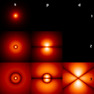
The hydrogen atom is an example where both types of spectra appear. The eigenfunctions of the hydrogen atom Hamiltonian are called eigenstates and are grouped into two categories. The bound states of the hydrogen atom correspond to the discrete part of the spectrum (they have a discrete set of eigenvalues which can be computed by Rydberg formula) while the ionization processes are described by the continuous part (the energy of the collision/ionization is not quantized).

Eigenfunctions

A common example of such maps on infinite dimensional spaces are the action of differential operators on function spaces. As an example, on the space of infinitely differentiable functions, the process of differentiation defines a linear operator since

$\displaystyle\frac{d}{dt}(af+bg) = a \frac{df}{dt} + b \frac{dg}{dt},$

where f(t) and g(t) are differentiable functions, and a and b are constants.

The eigenvalue equation for linear differential operators is then a set of one or more differential equations. The eigenvectors are commonly called eigenfunctions. The most simple case is the eigenvalue equation for differentiation of a real valued function by a single real variable. We seek a function (equivalent to an infinite-dimensional vector) which, when differentiated, yields a constant times the original function. In this case, the eigenvalue equation becomes the linear differential equation

$\displaystyle\frac{d}{dx} f(x) = \lambda f(x).$

Here λ is the eigenvalue associated with the function, f(x). This eigenvalue equation has a solution for any value of λ. If λ is zero, the solution is

$f(x) = A,\,$

where A is any constant; if λ is non-zero, the solution is the exponential function

$f(x) = Ae^{\lambda x}.\$

If we expand our horizons to complex valued functions, the value of λ can be any complex number. The spectrum of d/dt is therefore the whole complex plane. This is an example of a continuous spectrum.

Waves on a string

The shape of a standing wave in a string fixed at its boundaries is an example of an eigenfunction of a differential operator. The admittable eigenvalues are governed by the length of the string and determine the frequency of oscillation.

The displacement, $h(x,t)$ , of a stressed rope fixed at both ends, like the vibrating strings of a string instrument, satisfies the wave equation

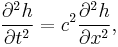
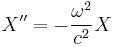
$\frac{\partial^2 h}{\partial t^2} = c^2\frac{\partial^2 h}{\partial x^2},$

which is a linear partial differential equation, where c is the constant wave speed. The normal method of solving such an equation is separation of variables. If we assume that h can be written as the product of the form X(x)T(t), we can form a pair of ordinary differential equations:

$X''=-\frac{\omega^2}{c^2}X$ and $T''=-\omega^2 T.\$

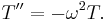
Each of these is an eigenvalue equation (the unfamiliar form of the eigenvalue is chosen merely for convenience). For any values of the eigenvalues, the eigenfunctions are given by

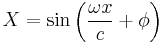$X = \sin \left(\frac{\omega x}{c} + \phi \right)\$ and $T = \sin(\omega t + \psi).\$

If we impose boundary conditions (that the ends of the string are fixed with X(x)=0 at x=0 and x=L, for example) we can constrain the eigenvalues. For those boundary conditions, we find

$\sin(\phi) = 0\$ , and so the phase angle $\phi=0\$

and

$\sin\left(\frac{\omega L}{c}\right) = 0.\$

Thus, the constant $\omega$ is constrained to take one of the values $\omega_n = \frac{nc\pi}{L}$ , where n is any integer. Thus the clamped string supports a family of standing waves of the form

$h(x,t) = \sin(n\pi x/L)\sin(\omega_n t).\$

From the point of view of our musical instrument, the frequency $\omega_n\$ is the frequency of the nth harmonic, which is called the (n-1)st overtone.

Eigendecomposition

The spectral theorem for matrices can be stated as follows. Let A be a square n × n matrix. Let q₁ ... q_k be an eigenvector basis, i.e. an indexed set of k linearly independent eigenvectors, where k is the dimension of the space spanned by the eigenvectors of A. If k = n, then A can be written

$\mathbf{A}=\mathbf{Q}\mathbf{\Lambda}\mathbf{Q}^{-1}$

where Q is the square n × n matrix whose i-th column is the basis eigenvector q_i of A and Λ is the diagonal matrix whose diagonal elements are the corresponding eigenvalues, i.e. Λ_ii = λ_i.

Applications

Schrödinger equation

The wavefunctions associated with the bound states of an electron in a hydrogen atom can be seen as the eigenvectors of the hydrogen atom Hamiltonian as well as of the angular momentum operator. They are associated with eigenvalues interpreted as their energies (increasing downward: n=1,2,3,...) and angular momentum (increasing across: s, p, d,...). The illustration shows the square of the absolute value of the wavefunctions. Brighter areas correspond to higher probability density for a position measurement. The center of each figure is the atomic nucleus, a proton.

An example of an eigenvalue equation where the transformation T is represented in terms of a differential operator is the time-independent Schrödinger equation in quantum mechanics:

$H\psi_E = E\psi_E \,$

where H, the Hamiltonian, is a second-order differential operator and $\psi_E$ , the wavefunction, is one of its eigenfunctions corresponding to the eigenvalue E, interpreted as its energy.

However, in the case where one is interested only in the bound state solutions of the Schrödinger equation, one looks for $\psi_E$ within the space of square integrable functions. Since this space is a Hilbert space with a well-defined scalar product, one can introduce a basis set in which $\psi_E$ and H can be represented as a one-dimensional array and a matrix respectively. This allows one to represent the Schrödinger equation in a matrix form.

Bra-ket notation is often used in this context. A vector, which represents a state of the system, in the Hilbert space of square integrable functions is represented by $|\Psi_E\rangle$ . In this notation, the Schrödinger equation is:

$H|\Psi_E\rangle = E|\Psi_E\rangle$

where $|\Psi_E\rangle$ is an eigenstate of H. It is a self adjoint operator, the infinite dimensional analog of Hermitian matrices (see Observable). As in the matrix case, in the equation above $H|\Psi_E\rangle$ is understood to be the vector obtained by application of the transformation H to $|\Psi_E\rangle$ .

Molecular orbitals

In quantum mechanics, and in particular in atomic and molecular physics, within the Hartree–Fock theory, the atomic and molecular orbitals can be defined by the eigenvectors of the Fock operator. The corresponding eigenvalues are interpreted as ionization potentials via Koopmans' theorem. In this case, the term eigenvector is used in a somewhat more general meaning, since the Fock operator is explicitly dependent on the orbitals and their eigenvalues. If one wants to underline this aspect one speaks of nonlinear eigenvalue problem. Such equations are usually solved by an iteration procedure, called in this case self-consistent field method. In quantum chemistry, one often represents the Hartree–Fock equation in a non-orthogonal basis set. This particular representation is a generalized eigenvalue problem called Roothaan equations.

Geology and glaciology

In geology, especially in the study of glacial till, eigenvectors and eigenvalues are used as a method by which a mass of information of a clast fabric's constituents' orientation and dip can be summarized in a 3-D space by six numbers. In the field, a geologist may collect such data for hundreds or thousands of clasts in a soil sample, which can only be compared graphically such as in a Tri-Plot (Sneed and Folk) diagram ^[22],^[23], or as a Stereonet on a Wulff Net ^[24]. The output for the orientation tensor is in the three orthogonal (perpendicular) axes of space. Eigenvectors output from programs such as Stereo32 ^[25] are in the order E₁ ≥ E₂ ≥ E₃, with E₁ being the primary orientation of clast orientation/dip, E₂ being the secondary and E₃ being the tertiary, in terms of strength. The clast orientation is defined as the eigenvector, on a compass rose of 360°. Dip is measured as the eigenvalue, the modulus of the tensor: this is valued from 0° (no dip) to 90° (vertical). The relative values of E₁, E₂, and E₃ are dictated by the nature of the sediment's fabric. If E₁ = E₂ = E₃, the fabric is said to be isotropic. If E₁ = E₂ > E₃ the fabric is planar. If E₁ > E₂ > E₃ the fabric is linear. See 'A Practical Guide to the Study of Glacial Sediments' by Benn & Evans, 2004 ^[26].

Principal components analysis

PCA of the multivariate Gaussian distribution centered at (1,3) with a standard deviation of 3 in roughly the (0.878, 0.478) direction and of 1 in the orthogonal direction.

Main article: Principal components analysis

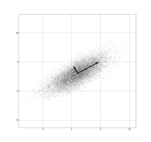
The eigendecomposition of a symmetric positive semidefinite (PSD) matrix yields an orthogonal basis of eigenvectors, each of which has a nonnegative eigenvalue. The orthogonal decomposition of a PSD matrix is used in multivariate analysis, where the sample covariance matrices are PSD. This orthogonal decomposition is called principal components analysis (PCA) in statistics. PCA studies linear relations among variables. PCA is performed on the covariance matrix or the correlation matrix (in which each variable is scaled to have its sample variance equal to one). For the covariance or correlation matrix, the eigenvectors correspond to principal components and the eigenvalues to the variance explained by the principal components. Principal component analysis of the correlation matrix provides an orthonormal eigen-basis for the space of the observed data: In this basis, the largest eigenvalues correspond to the principal-components that are associated with most of the covariability among a number of observed data.

Principal component analysis is used to study large data sets, such as those encountered in data mining, chemical research, psychology, and in marketing. PCA is popular especially in psychology, in the field of psychometrics. In Q-methodology, the eigenvalues of the correlation matrix determine the Q-methodologist's judgment of practical significance (which differs from the statistical significance of hypothesis testing): The factors with eigenvalues greater than 1.00 are considered to be practically significant, that is, as explaining an important amount of the variability in the data, while eigenvalues less than 1.00 are considered practically insignificant, as explaining only a negligible portion of the data variability. More generally, principal component analysis can be used as a method of factor analysis in structural equation modeling.

Vibration analysis

1st lateral bending (See vibration for more types of vibration)

Main article: Vibration

Eigenvalue problems occur naturally in the vibration analysis of mechanical structures with many degrees of freedom. The eigenvalues are used to determine the natural frequencies (or eigenfrequencies) of vibration, and the eigenvectors determine the shapes of these vibrational modes. The orthogonality properties of the eigenvectors allows decoupling of the differential equations so that the system can be represented as linear summation of the eigenvectors. The eigenvalue problem of complex structures is often solved using finite element analysis.

Eigenfaces

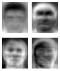
Eigenfaces as examples of eigenvectors

In image processing, processed images of faces can be seen as vectors whose components are the brightnesses of each pixel.^[27] The dimension of this vector space is the number of pixels. The eigenvectors of the covariance matrix associated with a large set of normalized pictures of faces are called eigenfaces; this is an example of principal components analysis. They are very useful for expressing any face image as a linear combination of some of them. In the facial recognition branch of biometrics, eigenfaces provide a means of applying data compression to faces for identification purposes. Research related to eigen vision systems determining hand gestures has also been made.

Similar to this concept, eigenvoices represent the general direction of variability in human pronunciations of a particular utterance, such as a word in a language. Based on a linear combination of such eigenvoices, a new voice pronunciation of the word can be constructed. These concepts have been found useful in automatic speech recognition systems, for speaker adaptation.

Tensor of inertia

In mechanics, the eigenvectors of the inertia tensor define the principal axes of a rigid body. The tensor of inertia is a key quantity required in order to determine the rotation of a rigid body around its center of mass.

Stress tensor

In solid mechanics, the stress tensor is symmetric and so can be decomposed into a diagonal tensor with the eigenvalues on the diagonal and eigenvectors as a basis. Because it is diagonal, in this orientation, the stress tensor has no shear components; the components it does have are the principal components.

Eigenvalues of a graph

In spectral graph theory, an eigenvalue of a graph is defined as an eigenvalue of the graph's adjacency matrix A, or (increasingly) of the graph's Laplacian matrix, which is either T−A (sometimes called the Combinatorial Laplacian) or I−T ^-1/2AT ^−1/2 (sometimes called the Normalized Laplacian), where T is a diagonal matrix with T_{v, v} equal to the degree of vertex v, and in T ^−1/2, the v, vth entry is deg(v)^-1/2. The kth principal eigenvector of a graph is defined as either the eigenvector corresponding to the kth largest or kth smallest eigenvalue of the Laplacian. The first principal eigenvector of the graph is also referred to merely as the principal eigenvector.

The principal eigenvector is used to measure the centrality of its vertices. An example is Google's PageRank algorithm. The principal eigenvector of a modified adjacency matrix of the World Wide Web graph gives the page ranks as its components. This vector corresponds to the stationary distribution of the Markov chain represented by the row-normalized adjacency matrix; however, the adjacency matrix must first be modified to ensure a stationary distribution exists. The second smallest eigenvector can be used to partition the graph into clusters, via spectral clustering. Other methods are also available for clustering.

Notes

↑ See also: eigen or eigenvalue at Wiktionary.
↑ http://mathworld.wolfram.com/Eigenvector.html
↑ See Korn & Korn 2000, Section 14.3.5a; Friedberg, Insel & Spence 1989, p. 217
↑ Axler, Sheldon Linear Algebra Done Right 2nd Edition, Ch. 5, page 77
↑ ^5.0 ^5.1 ^5.2 Lloyd N. Trefethen and David Bau, Numerical Linear Algebra (SIAM, 1997)
↑ For a proof of this lemma, see Shilov 1977, p. 109, and Lemma for the eigenspace
↑ For a proof of this lemma, see Roman 2008, Theorem 8.2 on p. 186; Shilov 1977, p. 109; Hefferon 2001, p. 364; Beezer 2006, Theorem EDELI on p. 469; and Lemma for linear independence of eigenvectors
↑ See Shilov 1977, p. 109
↑ Gilbert Strang, Linear Algebra and Its Applications, 3rd ed. (Harcourt: San Diego, 1988).
↑ See Hawkins 1975, §2
↑ ^11.0 ^11.1 ^11.2 ^11.3 See Hawkins 1975, §3
↑ ^12.0 ^12.1 ^12.2 See Kline 1972, pp. 807-808
↑ See Kline 1972, p. 673
↑ See Kline 1972, pp. 715-716
↑ See Kline 1972, pp. 706-707
↑ See Kline 1972, p. 1063
↑ See Aldrich 2006
↑ J.G.F. Francis, "The QR Transformation, I" (part 1), The Computer Journal, vol. 4, no. 3, pages 265-271 (1961); "The QR Transformation, II" (part 2), The Computer Journal, vol. 4, no. 4, pages 332-345 (1962).
↑ Vera N. Kublanovskaya, "On some algorithms for the solution of the complete eigenvalue problem" USSR Computational Mathematics and Mathematical Physics, vol. 3, pages 637–657 (1961). Also published in: Zhurnal Vychislitel'noi Matematiki i Matematicheskoi Fiziki, vol.1, no. 4, pages 555–570 (1961).
↑ See Golub & van Loan 1996, §7.3; Meyer 2000, §7.3
↑ Definition according to Weisstein, Eric W. Shear From MathWorld − A Wolfram Web Resource
↑ Graham, D., and Midgley, N., 2000. Earth Surface Processes and Landforms (25) pp 1473-1477
↑ Sneed ED, Folk RL. 1958. Pebbles in the lower Colorado River, Texas, a study of particle morphogenesis. Journal of Geology 66(2): 114–150
↑ GIS-stereoplot: an interactive stereonet plotting module for ArcView 3.0 geographic information system
↑ Stereo32
↑ Benn, D., Evans, D., 2004. A Practical Guide to the study of Glacial Sediments. London: Arnold. pp 103-107
↑ Xirouhakis, A.; Votsis, G.; Delopoulus, A. (2004) (PDF), Estimation of 3D motion and structure of human faces, Online paper in PDF format, National Technical University of Athens, http://www.image.ece.ntua.gr/papers/43.pdf

References

Korn, Granino A.; Korn, Theresa M. (2000), Mathematical Handbook for Scientists and Engineers: Definitions, Theorems, and Formulas for Reference and Review, 1152 p., Dover Publications, 2 Revised edition, ISBN 0-486-41147-8 .
Lipschutz, Seymour (1991), Schaum's outline of theory and problems of linear algebra, Schaum's outline series (2nd ed.), New York, NY: McGraw-Hill Companies, ISBN 0-07-038007-4 .
Friedberg, Stephen H.; Insel, Arnold J.; Spence, Lawrence E. (1989), Linear algebra (2nd ed.), Englewood Cliffs, NJ 07632: Prentice Hall, ISBN 0-13-537102-3 .
Aldrich, John (2006), "Eigenvalue, eigenfunction, eigenvector, and related terms", in Jeff Miller (Editor), Earliest Known Uses of Some of the Words of Mathematics, http://jeff560.tripod.com/e.html, retrieved 2006-08-22
Strang, Gilbert (1993), Introduction to linear algebra, Wellesley-Cambridge Press, Wellesley, MA, ISBN 0-961-40885-5 .
Strang, Gilbert (2006), Linear algebra and its applications, Thomson, Brooks/Cole, Belmont, CA, ISBN 0-030-10567-6 .
Bowen, Ray M.; Wang, Chao-Cheng (1980), Linear and multilinear algebra, Plenum Press, New York, NY, ISBN 0-306-37508-7 .
Cohen-Tannoudji, Claude (1977), "Chapter II. The mathematical tools of quantum mechanics", Quantum mechanics, John Wiley & Sons, ISBN 0-471-16432-1 .
Fraleigh, John B.; Beauregard, Raymond A. (1995), Linear algebra (3rd ed.), Addison-Wesley Publishing Company, ISBN 0-201-83999-7 (international edition) .
Golub, Gene H.; Van Loan, Charles F. (1996), Matrix computations (3rd Edition), Johns Hopkins University Press, Baltimore, MD, ISBN 978-0-8018-5414-9 .
Hawkins, T. (1975), "Cauchy and the spectral theory of matrices", Historia Mathematica 2: 1–29, doi:10.1016/0315-0860(75)90032-4 .
Horn, Roger A.; Johnson, Charles F. (1985), Matrix analysis, Cambridge University Press, ISBN 0-521-30586-1 (hardback), ISBN 0-521-38632-2 (paperback) .
Kline, Morris (1972), Mathematical thought from ancient to modern times, Oxford University Press, ISBN 0-195-01496-0 .
Meyer, Carl D. (2000), Matrix analysis and applied linear algebra, Society for Industrial and Applied Mathematics (SIAM), Philadelphia, ISBN 978-0-89871-454-8 .
Brown, Maureen (October 2004), Illuminating Patterns of Perception: An Overview of Q Methodology .
Golub, Gene F.; van der Vorst, Henk A. (2000), "Eigenvalue computation in the 20th century", Journal of Computational and Applied Mathematics 123: 35–65, doi:10.1016/S0377-0427(00)00413-1 .
Akivis, Max A.; Vladislav V. Goldberg (1969), Tensor calculus, Russian, Science Publishers, Moscow .
Gelfand, I. M. (1971), Lecture notes in linear algebra, Russian, Science Publishers, Moscow .
Alexandrov, Pavel S. (1968), Lecture notes in analytical geometry, Russian, Science Publishers, Moscow .
Carter, Tamara A.; Tapia, Richard A.; Papaconstantinou, Anne, Linear Algebra: An Introduction to Linear Algebra for Pre-Calculus Students, Rice University, Online Edition, http://ceee.rice.edu/Books/LA/index.html, retrieved 2008-02-19 .
Roman, Steven (2008), Advanced linear algebra (3rd ed.), New York, NY: Springer Science + Business Media, LLC, ISBN 978-0-387-72828-5 .
Shilov, Georgi E. (1977), Linear algebra (translated and edited by Richard A. Silverman ed.), New York: Dover Publications, ISBN 0-486-63518-X .
Hefferon, Jim (2001), Linear Algebra, Online book, St Michael's College, Colchester, Vermont, USA, http://joshua.smcvt.edu/linearalgebra/ .
Kuttler, Kenneth (2007) (PDF), An introduction to linear algebra, Online e-book in PDF format, Brigham Young University, http://www.math.byu.edu/~klkuttle/Linearalgebra.pdf .
Demmel, James W. (1997), Applied numerical linear algebra, SIAM, ISBN 0-89871-389-7 .
Beezer, Robert A. (2006), A first course in linear algebra, Free online book under GNU licence, University of Puget Sound, http://linear.ups.edu/ .
Lancaster, P. (1973), Matrix theory, Russian, Moscow, Russia: Science Publishers .
Halmos, Paul R. (1987), Finite-dimensional vector spaces (8th ed.), New York, NY: Springer-Verlag, ISBN 0387900934 .
Pigolkina, T. S. and Shulman, V. S., Eigenvalue (in Russian), In:Vinogradov, I. M. (Ed.), Mathematical Encyclopedia, Vol. 5, Soviet Encyclopedia, Moscow, 1977.
Greub, Werner H. (1975), Linear Algebra (4th Edition), Springer-Verlag, New York, NY, ISBN 0-387-90110-8 .
Larson, Ron; Edwards, Bruce H. (2003), Elementary linear algebra (5th ed.), Houghton Mifflin Company, ISBN 0-618-33567-6 .
Curtis, Charles W., Linear Algebra: An Introductory Approach, 347 p., Springer; 4th ed. 1984. Corr. 7th printing edition (August 19, 1999), ISBN 0-387-90992-3.
Shores, Thomas S. (2007), Applied linear algebra and matrix analysis, Springer Science+Business Media, LLC, ISBN 0-387-33194-8 .
Sharipov, Ruslan A. (1996), Course of Linear Algebra and Multidimensional Geometry: the textbook, Online e-book in various formats on arxiv.org, Bashkir State University, Ufa, arXiv:math/0405323v1, ISBN 5-7477-0099-5, http://arxiv.org/pdf/math/0405323v1 .
Gohberg, Israel; Lancaster, Peter; Rodman, Leiba (2005), Indefinite linear algebra and applications, Basel-Boston-Berlin: Birkhäuser Verlag, ISBN 3-7643-7349-0 .

External links

What are Eigen Values? — non-technical introduction from PhysLink.com's "Ask the Experts"
Introduction to Eigen Vectors and Eigen Values -- lecture from Kahn Academy

Theory

Eigenvalue (of a matrix) on PlanetMath
Eigenvector — Wolfram MathWorld
Eigen Vector Examination working applet
Same Eigen Vector Examination as above in a Flash demo with sound
Computation of Eigenvalues
Numerical solution of eigenvalue problems Edited by Zhaojun Bai, James Demmel, Jack Dongarra, Axel Ruhe, and Henk van der Vorst
Eigenvalues and Eigenvectors on the Ask Dr. Math forums: [1], [2]

Algorithms

ARPACK is a collection of FORTRAN subroutines for solving large scale (sparse) eigenproblems.
IRBLEIGS, has MATLAB code with similar capabilities to ARPACK. (See this paper for a comparison between IRBLEIGS and ARPACK.)
LAPACK is a collection of FORTRAN subroutines for solving dense linear algebra problems
ALGLIB includes a partial port of the LAPACK to C++, C#, Delphi, etc.
Vanderplaats Research and Development - Provides the SMS eigenvalue solver for Structural Finite Element. The solver is in the GENESIS program as well as other commercial programs. SMS can be easily use with MSC.Nastran or NX/Nastran via DMAPs.

Online calculators

Topics related to linear algebra

Scalar · Vector · Vector space · Vector projection · Linear span · Linear map · Linear projection · Linear independence · Linear combination · Basis · Column space · Row space · Dual space · Orthogonality · Rank · Minor · Kernel (matrix) · Eigenvalue, eigenvector and eigenspace · Least squares regressions · Outer product · Inner product space · Dot product · Transpose · Gram–Schmidt process · Matrix decomposition

Areas of mathematics

Arithmetic · Logic · Set theory · Combinatorics · Algebra (elementary – linear – abstract) · Number theory · Analysis/Calculus · Geometry · Topology · Statistics · Differential equations/Dynamical systems · Mathematical physics · Numerical analysis · Computation · Information theory · Probability · Optimization · Game theory

Category · Mathematics portal · Outline · Lists